INTRODUCTION TO DATA SCIENCE WITH R
INDEX
Program 1:
Basic Operations of R and sample programs on Arithmetic Operations
Program:
var1=c(4,5)
var2=c(2,4)
print("addition of two vectors")
print(var1+var2)
print("subtraction of two vectors")
print(var1-var2)
print("multiplication of two vectors")
print(var1*var2)
print("division of two vectors")
print(var1/var2)
print("modulous of two vectors")
print(var1%%var2)
Output:
[1] "addition of two vectors"
[1] 6 9
[1] "subtraction of two vectors"
[1] 2 1
[1] "multiplication of two vectors"
[1] 8 20
[1] "division of two vectors"
[1] 2.00 1.25
[1] "modulous of two vectors"
[1] 0 1
Program 2:
Basic programs of R and Sample Programs on Arithmetic Operations on vectors-II
1. Floor Division
2. Exponent
Program:
print("Floor Division of two vectors")
print(var1%/%var2)
print("Exponent")
print(var1^var2)
Output
[1] "Floor Division of two vectors"
[1] 2 1
[1] "Exponent"
[1] 16 625
Program 3
Operation on Matrix: Addition
Program:
A=matrix(c(3,5,4,6,7,8,9,3,5),nrow=3, ncol=3, byrow=TRUE)
print("First 3x3 matrix")
print(A)
B=matrix(c(5,6,7,2,4,3,6,9,7),nrow=3, ncol=3, byrow=TRUE)
print("Second 3x3 matrix")
print(B)
print("result of addition of two matrices")
print(A+B)
Output:
[1] "3x3 matrix"
[,1] [,2] [,3]
[1,] 3 5 4
[2,] 6 7 8
[3,] 9 3 5
[1] "3x3 matrix"
[,1] [,2] [,3]
[1,] 5 6 7
[2,] 2 4 3
[3,] 6 9 7
[1] "result of addition"
[,1] [,2] [,3]
[1,] 8 11 11
[2,] 8 11 11
[3,] 15 12 12
Subtraction of Two matrices
print("result of subtraction of two matrices")
print(A-B)
Output:
[1] "First 3x3 matrix"
[,1] [,2] [,3]
[1,] 3 5 4
[2,] 6 7 8
[3,] 9 3 5
[1] "Second 3x3 matrix"
[,1] [,2] [,3]
[1,] 5 6 7
[2,] 2 4 3
[3,] 6 9 7
[1] "result of subtraction of two matrices"
[,1] [,2] [,3]
[1,] -2 -1 -3
[2,] 4 3 5
[3,] 3 -6 -2
Multiplication of Two matrices
print("result of multiplication of two matrices")
print(A*B)
Output:
[1] "First 3x3 matrix"
[,1] [,2] [,3]
[1,] 3 5 4
[2,] 6 7 8
[3,] 9 3 5
[1] "Second 3x3 matrix"
[,1] [,2] [,3]
[1,] 5 6 7
[2,] 2 4 3
[3,] 6 9 7
[1] "result of multiplication of two matrices"
[,1] [,2] [,3]
[1,] 15 30 28
[2,] 12 28 24
[3,] 54 27 35
Division of Two matrices
print("result of division of two matrices")
print(A/B)
Output:
[1] "First 3x3 matrix"
[,1] [,2] [,3]
[1,] 3 5 4
[2,] 6 7 8
[3,] 9 3 5
[1] "Second 3x3 matrix"
[,1] [,2] [,3]
[1,] 5 6 7
[2,] 2 4 3
[3,] 6 9 7
[1] "result of division of two matrices"
[,1] [,2] [,3]
[1,] 0.6 0.8333333 0.5714286
[2,] 3.0 1.7500000 2.6666667
[3,] 1.5 0.3333333 0.7142857
Program 4:
Row Concatenation of two matrices
print("result of row concatenation of two matrices")
print(rbind(A,B))
Output:
[1] "First 3x3 matrix"
[,1] [,2] [,3]
[1,] 3 5 4
[2,] 6 7 8
[3,] 9 3 5
[1] "Second 3x3 matrix"
[,1] [,2] [,3]
[1,] 5 6 7
[2,] 2 4 3
[3,] 6 9 7
[1] "result of row concatenation of two matrices"
[,1] [,2] [,3]
[1,] 3 5 4
[2,] 6 7 8
[3,] 9 3 5
[4,] 5 6 7
[5,] 2 4 3
[6,] 6 9 7
Deleting Second Column
A=matrix(c(3,5,4,6,7,8,9,3,5),nrow=3, ncol=3, byrow=TRUE)
print("Before deleting Second column")
print(A)
A=A[,-2]
print("After deleting Second column")
print(A)
Output:
[1] "Before deleting Second column"
[,1] [,2] [,3]
[1,] 3 5 4
[2,] 6 7 8
[3,] 9 3 5
[1] "After deleting Second column"
[,1] [,2]
[1,] 3 4
[2,] 6 8
[3,] 9 5
Deleting Second Row
A=matrix(c(3,5,4,6,7,8,9,3,5),nrow=3, ncol=3, byrow=TRUE)
print("Before deleting Second Row")
print(A)
A=A[-2,]
print("After deleting Second Row")
print(A)
Output:
[1] "Before deleting Second Row"
[,1] [,2] [,3]
[1,] 3 5 4
[2,] 6 7 8
[3,] 9 3 5
[1] "After deleting Second Row"
[,1] [,2] [,3]
[1,] 3 5 4
[2,] 9 3 5
Updating Second Row
A=matrix(c(3,5,4,6,7,8,9,3,5),nrow=3, ncol=3, byrow=TRUE)
print("Before updating Second Row")
print(A)
A[2,]=c(11,12,15)
print("After updating Second Row")
print(A)
Output:
[1] "Before updating Second Row"
[,1] [,2] [,3]
[1,] 3 5 4
[2,] 6 7 8
[3,] 9 3 5
[1] "After updating Second Row"
[,1] [,2] [,3]
[1,] 3 5 4
[2,] 11 12 15
[3,] 9 3 5
Program 5:
Line Graph
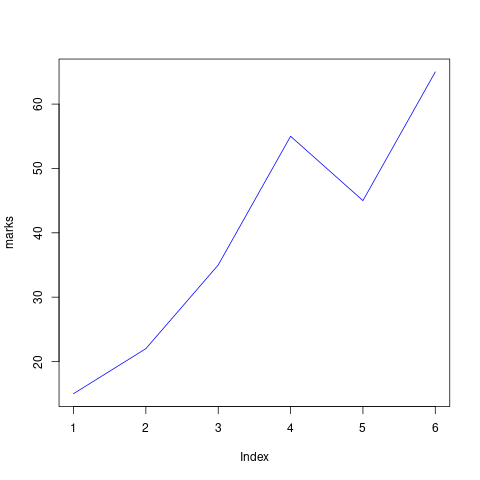
A line chart is a graph that connects a series of points by drawing line segments between them. These points are ordered in one of their coordinate (usually the x-coordinate) value. Line charts are usually used in identifying the trends in data.
The plot() function in R is used to create the line graph.
Syntax
The basic syntax to create a line chart in R is –
plot(v,type,col,xlab,ylab)
Following is the description of the parameters used −
v is a vector containing the numeric values.
type takes the value "p" to draw only the points, "l" to draw only the lines and "o" to draw both points and lines.
xlab is the label for x axis.
ylab is the label for y axis.
main is the Title of the chart.
col is used to give colors to both the points and lines.
Program:
marks=c(15,22,35,55,45,65)
plot(marks, type="l", col="Blue")
Output:
Program2:
marks=c(15,22,35,55,45,65)
plot(marks,type = "o", col = "red", xlab = "Roll Number", ylab = "Marks in Statistics",
main = "Marks Obtained by Data Science Students")
Output

Bell Curves
1. First we generate normal distributed data using rnorm function
Syntax of rnorm function in R:
rnorm(n, mean, sd)
n: It is the number of observations(sample size).
mean: It is the mean value of the sample data. Its default value is zero.
sd: It is the standard deviation. Its default value is 1.
Program
n=floor(rnorm(10000,500,100))
t=table(n)
plot(t)
Output:

Program 6:
Bar Chart
Program:
marks=c(92,50,45,73)
barplot(marks, main="Comparing marks of 5 subjects", xlab="marks", ylab="subjects", names.arg = c("eng","comp","math"," r program"), col="blue",horiz=FALSE)
Output:

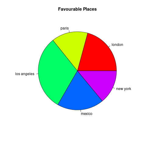
Pie Chart
Syntax:
The basic syntax for creating a pie-chart using the R is −
pie(x, labels, radius, main, col, clockwise)
Following is the description of the parameters used −
x is a vector containing the numeric values used in the pie chart.
labels is used to give description to the slices.
radius indicates the radius of the circle of the pie chart.(value between −1 and +1).
main indicates the title of the chart.
col indicates the color palette.
clockwise is a logical value indicating if the slices are drawn clockwise or anti clockwise.
Program
vtr=c(43,31,64,40,29)
names=c("london","paris","los angeles", "mexico","new york")
pie(vtr,labels=names,main="Favourable Places", col= rainbow(length(vtr)))
Output:
Program 7:
There are three types of loop in R programming:
for
while
repeat
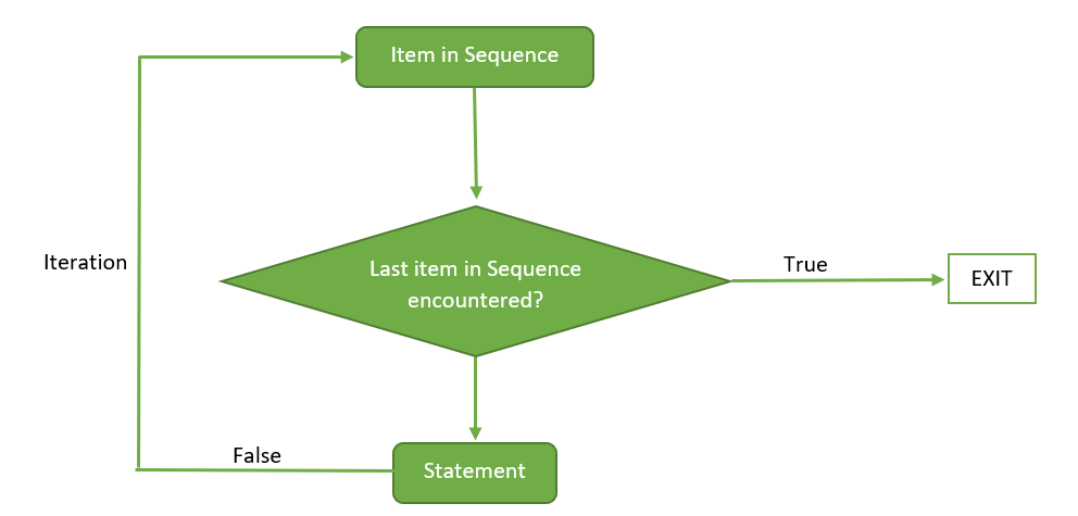
1. for loop
Syntax:
for (value in sequence)
{
statement
}
Flow Chart:
Program to print first five natural numbers:
for (i in 1:5)
{
# statement
print(i)
}
Output:
[1] 1
[1] 2
[1] 3
[1] 4
[1] 5
Program to display days of week using for loop
week = c('Sunday', 'Monday','Tuesday', 'Wednesday', 'Thursday', 'Friday', 'Saturday')
for (day in week)
{
print(day)
}
Output:
[1] "Sunday"
[1] "Monday"
[1] "Tuesday"
[1] "Wednesday"
[1] "Thursday"
[1] "Friday"
[1] "Saturday"
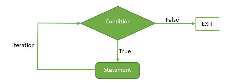
While loop
Syntax:
while( condition)
{
statement
}
Flow chart:
Program to calculate factorial of 5.
n=5
factorial = 1
i = 1
while (i <= n)
{
factorial = factorial * i
i = i + 1
}
print(factorial)
Output:
[1] 120
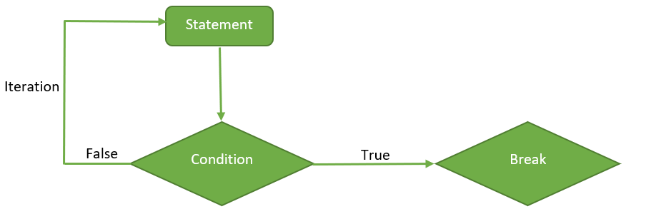
Repeat Loop
Repeat loop does not have any condition to terminate the loop, a programmer must specifically place a condition within the loop’s body and use the declaration of a break statement to terminate this loop. If no condition is present in the body of the repeat loop then it will iterate infinitely.
Syntax:
repeat
{
statement
if( condition )
{
break
}
}
Flow chart:
Program:
Program to display numbers from 1 to 5 using repeat loop in R.
val = 1
repeat
{
print(val)
val = val + 1
if(val > 5)
{
break
}
}
Output:
[1] 1
[1] 2
[1] 3
[1] 4
[1] 5
Program 8: Functions in R
Function Components
The different parts of a function are −
Function Name − This is the actual name of the function. It is stored in R environment as an object with this name.
Arguments − An argument is a placeholder. When a function is invoked, you pass a value to the argument. Arguments are optional; that is, a function may contain no arguments. Also arguments can have default values.
Function Body − The function body contains a collection of statements that defines what the function does.
Return Value − The return value of a function is the last expression in the function body to be evaluated.
R has many in-built functions which can be directly called in the program without defining them first. We can also create and use our own functions referred as user defined functions.
Built-in Function
Simple examples of in-built functions are seq(), mean(), max(), sum(x) and paste(...) etc. They are directly called by user written programs. You can refer most widely used R functions.
# Create a sequence of numbers from 32 to 44.
print(seq(32,44))
# Find mean of numbers from 25 to 82.
print(mean(25:82))
# Find sum of numbers frm 41 to 68.
print(sum(41:68))
User-defined Function
We can create user-defined functions in R. They are specific to what a user wants and once created they can be used like the built-in functions. Below is an example of how a function is created and used.
Program to create a function to print squares of first n natural numbers
No comments:
Post a Comment