Define Data science
Data science is the area of study which involves extracting knowledge from all the data you can gather. Here we are translating a business problem into a research problem and then translating result back into a practical solution. People doing all this are called data scientist.
Data Science Life Cycle
Step 1: Define Problem Statement: In meeting with clients, data scientist must ask relevant questions to understand and define objectives of the problem that need to be tackled.
Step 2: Data Collection: If there is no data available, then, you need to collect new data. This method is called as primary data collection.
Another method is to use the data which is readily available. This is called secondary data collection. Here raw data is gathered from multiple sources like flat files and online repositories etc
The data collected need to be prepared for extracting knowledge
Step 3: Data preparation: The most essential part of any data science project is data preparation. It consumes 60% of the time spent on the project.
Steps in data preparation are
1. Data cleaning: It handles missing values, NULL or unwanted values, duplicate values, misspelled attributes, inconsistent data types.
2. Data transformation: turns raw data formats into desired outputs. It also normalizes the data.
3. Handling outliers: Outliers are observations which are distant from the rest of the data. Outliers can be good or bad for the data. Outliers can be used for fraud detection. Scatter plots and box plots help to identify the outliers in the data.
4. Data integration: When data from multiple sources are integrated, the data after integration must be accurate and reliable. Primary keys and foreign keys are handled while integrating data.
5. Data reduction: Here we reduce the size of data by eliminating duplicate columns etc..
Step 4: Data mining or Exploratory Data Analysis (EDA):
EDA helps us understand what we can actually do with the data. EDA helps understand the relationships between data and helps us in selecting the variables that will be used in model development. It also helps us in identifying the right algorithm.
Softwares available: tableau
Step 5: Model building: The model is built by selecting a machine learning algorithm that suits the data. Regression is used to predict continuous values
Example: predicting house prices, temperature etc..
and classification is used to predict discrete values. Example: classifying whether the email is spam or not. Customer will buy a product or not.
For modeling the data, we can use the tools: R , python or SAS
Step 6: Visualization and communication: the business finding are communicated to business clients using simple and effective manner to convince the client. The visualization tools like tableau, powerBi, QlikView can be used to create powerful reports and dashboards
What is R program used for?
R program is used for
Statistical inference
Data analysis
Machine learning algorithm
R has multiple ways to present and share work, either through a markdown document or a shiny app. Everything can be hosted in Rpub, GitHub or the business’s website.
Rstudio accepts markdown to write a document. You can export the documents in different formats:
Document :
HTML
PDF/Latex
Word
Presentation
HTML
PDF beamer
What are the different types of data in Data science.
Flat Files
Relational Databases
DataWarehouse
Transactional Databases
Multimedia Databases
Spatial Databases
Time Series Databases
World Wide Web(WWW)
Flat Files
Flat files is defined as data files in text form or binary form with a structure
Data stored in flat files have no relations between them.
Eg: CSV file.
Application: Used in DataWarehousing to store data, Used in carrying data to and from server, etc.
Relational Databases
A Relational database is defined as the collection of tables
Physical schema in Relational databases is a schema which defines the structure of tables.
Logical schema in Relational databases is a schema which defines the relationship among tables.
Ex: SQL.
Application: Data Mining etc.
DataWarehouse
A datawarehouse is defined as the collection of data integrated from multiple sources that will queries and decision making.
Application: Business decision making, Data mining, etc.
Transactional Databases
Transactional databases is a collection of data organized by time stamps, date, etc to represent transaction in databases.
This type of database has the capability to roll back or undo its operation when a transaction is not completed or committed.
Highly flexible system where users can modify information without changing any sensitive information.
Application: Bank Transaction Data etc.
Multimedia Databases
Multimedia databases consists audio, video, images and text media.
They can be stored on Object-Oriented Databases.
They are used to store complex information in a pre-specified formats.
Application: Digital libraries, video-on demand, news-on demand, musical database, etc.
Spatial Database
Store geographical information.
Stores data in the form of coordinates, topology, lines, polygons, etc.
Application: Maps, Global positioning, etc.
Time-series Databases
Time series databases contains stock exchange data and user logged activities.
Handles array of numbers indexed by time, date, etc.
It requires real-time analysis.
Application: eXtremeDB, Graphite, InfluxDB, etc.
WWW
WWW refers to World wide web is a collection of documents and resources like audio, video, text, etc which are identified by Uniform Resource Locators (URLs) through web browsers, linked by HTML pages, and accessible via the Internet network.
It is the most heterogeneous repository as it collects data from multiple resources.
It is dynamic in nature as Volume of data is continuously increasing and changing.
Application: Online shopping, Job search, Research, studying, etc.
What is Data Modeling.
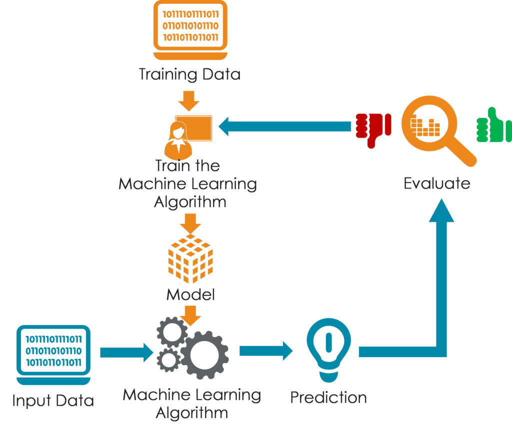
To predict something useful from the datasets, we need to implement machine learning algorithms like KNN, decision trees, Naïve Bayes. We repetitively apply diverse machine learning algorithms to identify the model that best fits the business requirement. The model is trained on training data set and the model is tested on test data. This testing is done to select the best performing model. The best trained model is then used to predict future or unknown data.
Regression is used to predict continuous values
Example: predicting house prices, temperature etc..
and classification is used to predict discrete values. Example: classifying whether the email is spam or not. Customer will buy a product or not.
Write common Vector operations in R.
Explain about data frames in R Language.
Data frame is collection of vectors of same size. A data frame is a table or a two-dimensional array-like structure in which each column contains values of one variable and each row contains one set of values from each column.
To create a data frame using data.frame() function:
v1=c(1,2,3,4,NA,6,7)
v2=c("pritam","nag","raju","srinu","kiran","xyz","abc")
v3=c(95,96,98,100,99,20,NA)
df=data.frame(v1,v2,v3)
Giving names to columns:
colnames(df)<- c("Roll","Student Names","marks")
Calculate average marks obtained by all students:
print(mean(df$marks))
To display first 6 rows in data frame
head(df)
To display last 6 rows in data frame:
tail(df)
To print the structure of data frame
str(df)
To print the statistical summary like min, max, mean, median, first quartile and 3rd quartile
summary(df)
To convert matrix to dataframe using as.data.frame() function
m1=matrix(c(9,78,6,4),2,2)
class(m1)
df2=as.data.frame(m1)
Explain General List Operations.
Vectors can only store on type of data. So, to overcome this limitation, we can use lists to store data of different types
Lists in R language, are the objects which comprise elements of diverse types like numbers, strings, logical values, vectors, list within a list and also matrix
Creating a list: Using list() function
list1= list("mango",50.25, TRUE)
print(list1)
Ouput:
[[1]]
[1] "mango"
These are levels of list
[[2]]
[1] 50.25
[[3]] To print this we need to type the code: print(list1[[1]][1]
[1] TRUE
Naming the elements of list:
list1= list("mango",50.25, TRUE)
names(list1)=c("Fruit","price","available")
print(list1)
Output:
$Fruit
[1] "mango"
$price
[1] 50.25
$available
[1] TRUE
Accessing elements of a List
In order to access the list elements, use the index number, and in case of named list, elements can be accessed using its name also.
Example :
print(list1[[2]][1])
Output:
[1] 50.25
Converting a list to vector using unlist() function
In order to perform arithmetic operations, lists should be converted to vectors using unlist() function.
Example:
v1=unlist(list1)
print(v1)
Output:
Fruit price available
"mango" "50.25" "TRUE"
a) Write an Overview of Data science
same as Question1 above
Explain Different data types in detail
same as Question 3 answer above
a)Explain types of Experimental Design
https://www.youtube.com/watch?v=10ikXret7Lk
Data for statistical studies are obtained by conducting either experiments or surveys. Experimental design is the branch of statistics that deals with the design and analysis of experiments. In an experimental study, variables of interest are identified. One or more of these variables are referred to as the factors of the study or independent variables. These variables influence another variable called response variable or dependent variable.
Three of the more widely used experimental designs are the completely randomized design, the randomized block design, and the matched pairs design
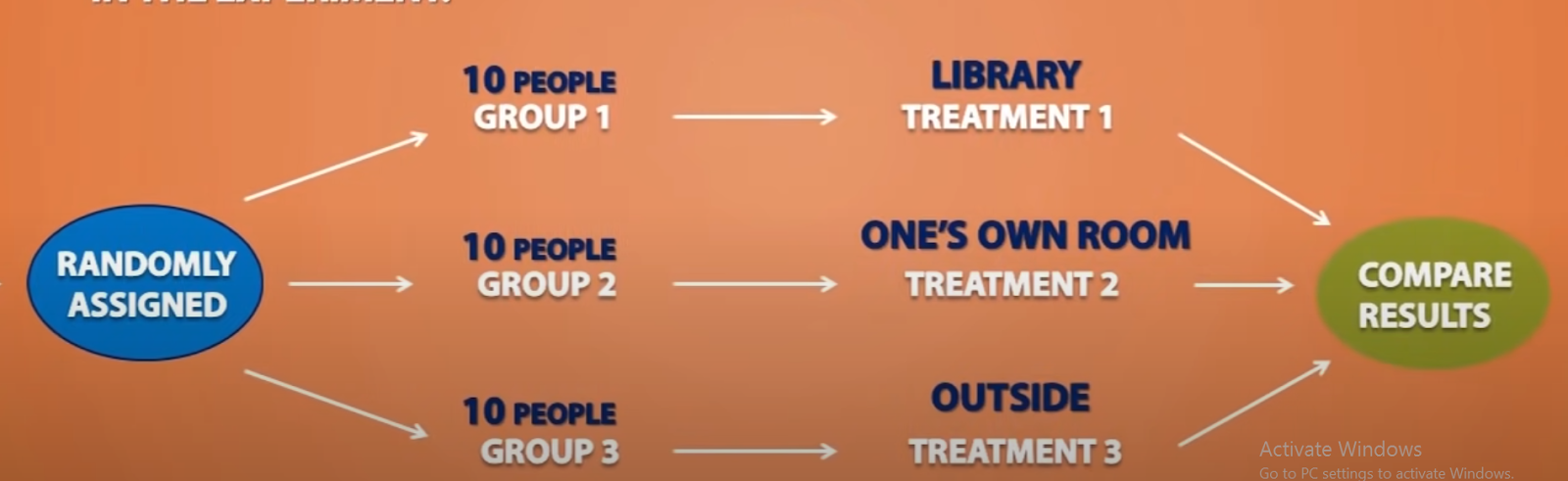
1. Completely randomized design:
Each experiment is randomly assigned to a random group to receive a different treatment. Each unit in same group will receive same treatment.
At the end of experiment, results from each treatment are compared.
For example: we need to find out which environment (library, one’s own room and outside) is best suited for studying. And 30 students from different universities volunteered to participate in this experiment.
Here in this experiment, there are 3 treatments
library
one’s own room
outside
We assign these 30 students randomly to 3 groups to receive treatments as shown below
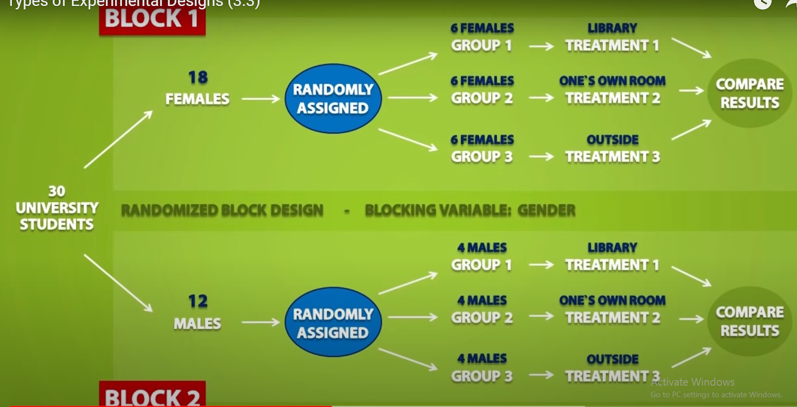
2. Randomized Block Design
If we feel gender has an effect on the results them we use randomized block design.
Here gender is blocking variable.
So first we separate our experimental units based on gender. One block for males and another for females.
Suppose there are 18 females and 12 males.
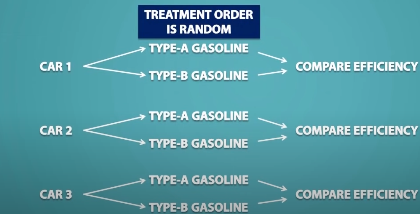
3. Matched Pairs Design
Here we compare two treatments using the same or similar experimental units
Suppose we need to find which type of gasoline is efficient, type A gasoline or type B gasoline.
3 cars will be used in this experiment.
Here each car will receive both the treatments, one with type A and one with type B. Same car would be used for each treatment and which treatment goes first will be random.
For example: first we fill the car with type B gasoline and once gasoline is finished, we would fill up the car with type A gasoline with same quantity. At the end of the experiment, we would compare the efficiency of gasoline.
There are cases where we cannot use the same experimental units for a matched pairs design,
Some more terminology:
Experiment – A procedure for investigating the effect of an experimental condition on a response variable.
Experimental units – Individuals on whom an experiment is performed (usually called subjects or participants).
Extraneous factor – A variable that is not of interest in the current study but is thought to affect the response variable.
Treatment – The process, intervention, or other controlled circumstance applied to randomly assigned experimental units.
Confounding variable - associated in a noncausal way with a factor and affects the response (usually found in experiments). Because of the confounding, we find that we can’t tell whether any effect we see was caused by our factor or by the confounding variable – or even both working together.
Direct control – Holding extraneous factors constant so that their effects are not
confounded with those of the experimental conditions.
For example, suppose we test two laundry detergents and carefully control the
water temperature at 180F. This would reduce the variation in our results due to water
temperature,
The best experiments are usually randomized, comparative, double-blind,
and placebo-controlled.
What are the steps involved in Data Cleaning. Explain in Detail
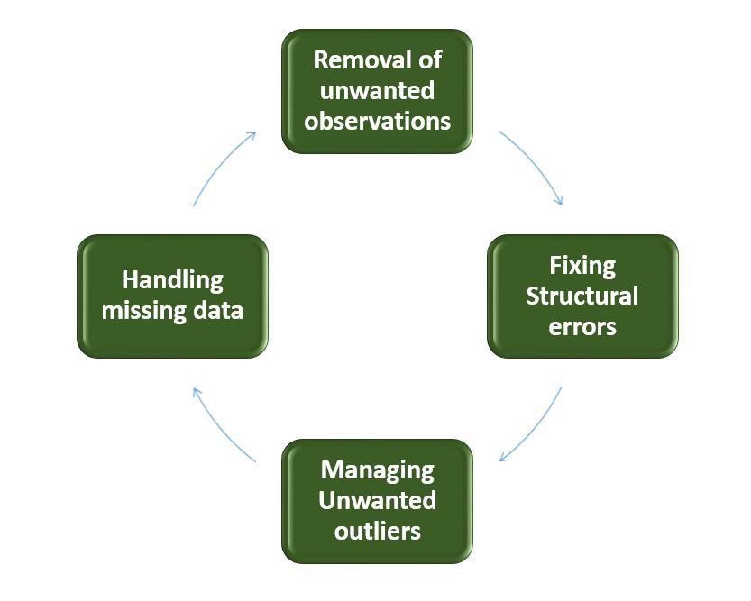
The success or failure of a project relies on proper data cleaning. Steps involved in Data Cleaning
Data cleaning tasks attempts to
1.Removal of unwanted data
2. Fixing Structural Errors
3. Managing unwanted outliers
4. Handling missing data
Removal of unwanted observations
This includes deleting duplicate/ redundant or irrelevant values from your dataset.
Irrelevant observations are any type of data that is of no use to us and can be removed directly.
2. Fixing Structural errors
The errors that arise during measurement, transfer of data, or other similar situations are called structural errors.
For example, the model will treat red, yellow, and red-yellow as different classes or attributes, though one class can be included in the other two classes. So, these are some structural errors that make our model inefficient and give poor quality results.
3. Managing Unwanted outliers
Outliers can cause problems with certain types of models. For example, linear regression models are less robust to outliers than decision tree models. Generally, we should not remove outliers until we have a good reason to remove them. Sometimes, removing them improves performance, sometimes not.
4. Handling missing data The two most common ways to deal with missing data are:
Dropping observations with missing values.
Fill in the missing value manually
Use a global constant to fill in the missing value: If all missing values are replaced by “unknown”, then mining program may mistakenly think that they form an interesting concept.
So this method is simple and not foolproof.
4. Use the attribute mean to fill in the missing value: For example, Use average income value to replace the missing value for income.
Some data cleansing tools
Openrefine
Trifacta Wrangler
TIBCO Clarity
Cloudingo
IBM Infosphere Quality Stage
a) Explain about ordered and unordered factors in R.
A factor is a vector object used to specify a discrete classification (grouping) of the components of other vectors of the same length. R provides both ordered and unordered factors.
Creating unordered factor using factor() function:
v1=c("pritham","nag","pritham","nag","nag")
f1=factor(v1)
print(f1)
Output:
[1] pritham nag pritham nag nag
Levels: nag pritham
To find out the levels of a factor the function levels() can be used.
levels(f1)
Output:
[1] "nag" "pritham"
Using tapply() to calculate mean of each level or student
Example: we create another vector fee that will store the fees paid at different times by pritham and nag
v1=c("pritham","nag","pritham","nag","nag")
fee=c(10,20,30,40,50)
f1=factor(v1)
total=tapply(fee,f1,sum)
print(total)
Output:
nag pritham
110 40
In R, there is a special data type for ordinal data. This type is called ordered factors and is an extension of factors that you’re already familiar with.
To create an ordered factor in R, you have two options:
Use the factor() function with the argument ordered=TRUE.
Use the ordered() function.
Example:
v1=c("pritham","nag","pritham","nag","nag")
f1=factor(v1,ordered=TRUE)
print(f1)
[1] pritham nag pritham nag nag
Levels: nag < pritham
You can tell an ordered factor from an ordinary factor by the presence of directional signs (< or >) in the levels.
b) Explain the different concepts of arrays in R Language or higher dimensional arrays in R
Arrays are the R objects which can store data in more than 2 dimensions.
For example, you make an array with four columns, three rows, and two “tables” like this:
> arr <- array(1:24, dim=c(3,4,2))
> print(arr)
, , 1
[,1] [,2] [,3] [,4]
[1,] 1 4 7 10
[2,] 2 5 8 11
[3,] 3 6 9 12
, , 2
[,1] [,2] [,3] [,4]
[1,] 13 16 19 22
[2,] 14 17 20 23
[3,] 15 18 21 24
This array has three dimensions. Notice that, although the rows are given as the first dimension, the tables are filled column-wise. So, for arrays, R fills the columns, then the rows, and then the rest.
Change the dimensions of a vector in R
Alternatively, you could just add the dimensions using the dim() function
If you already have a vector with the numbers 1 through 24, like this:
> v1 =c(1:24)
You can easily convert that vector to an array exactly like arr simply by assigning the dimensions, like this:
> dim(v1) <- c(3,4,2)
You can check whether two objects are identical by using the identical() function. To check, for example, whether my.vector and my.array are identical, you simply do the following:
> identical(arr,v1)
[1] TRUE
a) Explain about Poisson and normal distribution. or Explain about data distribution in R
https://www.youtube.com/watch?v=BbLfV0wOeyc
https://www.youtube.com/watch?v=778WK1Pf8eI
http://www.r-tutor.com/elementary-statistics/probability-distributions/normal-distribution
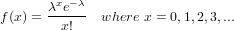
The Poisson distribution is the probability distribution of independent event occurrences in an interval. If λ is the mean occurrence per interval, then the probability of having x occurrences within a given interval is:
Problem
If there are twelve cars crossing a bridge per minute on average, find the probability of having seventeen or more cars crossing the bridge in a particular minute.
Solution
The probability of having sixteen or less cars crossing the bridge in a particular minute is given by the function ppois.
> ppois(16, lambda=12) # lower tail
[1] 0.89871
Hence the probability of having seventeen or more cars crossing the bridge in a minute is in the upper tail of the probability density function.
> ppois(16, lambda=12, lower=FALSE) # upper tail
[1] 0.10129
Answer
If there are twelve cars crossing a bridge per minute on average, the probability of having seventeen or more cars crossing the bridge in a particular minute is 10.1%.
Normal Distribution
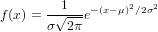
The normal distribution is defined by the following probability density function, where μ is the population mean and σ2 is the variance.
In particular, the normal distribution with μ = 0 and σ = 1 is called the standard normal distribution, and is denoted as N(0,1). It can be graphed as follows.
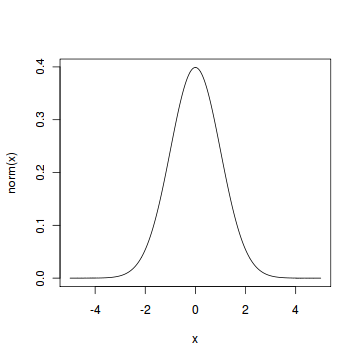
The normal distribution is important because of the Central Limit Theorem, which states that the population of all possible samples of size n from a population with mean μ and variance σ2 approaches a normal distribution with mean μ and σ2∕n when n approaches infinity.
Problem
Assume that the test scores of a college entrance exam fits a normal distribution. Furthermore, the mean test score is 72, and the standard deviation is 15.2. What is the percentage of students scoring 84 or more in the exam?
Solution
We apply the function pnorm of the normal distribution with mean 72 and standard deviation 15.2. Since we are looking for the percentage of students scoring higher than 84, we are interested in the upper tail of the normal distribution.
> pnorm(84, mean=72, sd=15.2, lower.tail=FALSE)
[1] 0.21492
Answer
The percentage of students scoring 84 or more in the college entrance exam is 21.5%.
a) Explain about graphical analysis.
Write about all the plots u did in lab
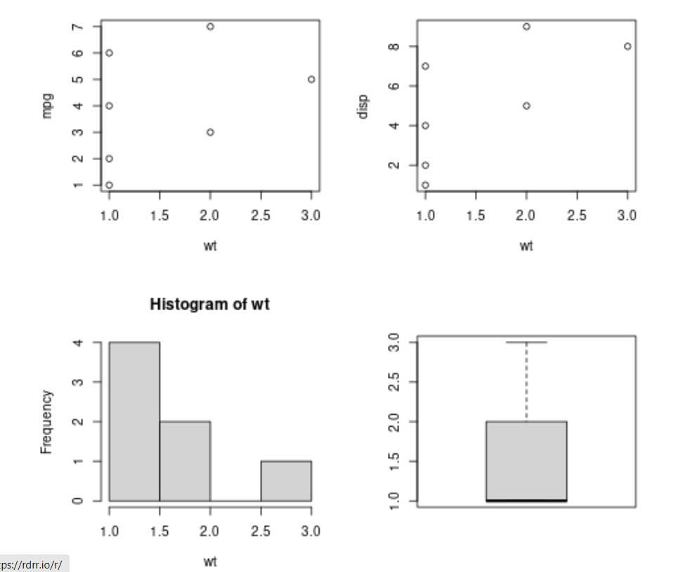
b) Explain about multiple plots in one window.
Combining Plots
R makes it easy to combine multiple plots into one overall graph, using either the
par( ) or layout( ) function.
With the par( ) function, you can include the option mfrow=c(nrows, ncols) to create a matrix of nrows x ncols plots that are filled in by row. mfcol=c(nrows, ncols) fills in the matrix by columns.
wt=c(1,1,2,1,3,1,2)
mpg=c(1,2,3,4,5,6,7)
disp=c(4,1,5,7,8,2,9)
par(mfrow=c(2,2))
plot(wt,mpg)
plot(wt,disp)
hist(wt)
boxplot(wt)
Output:
Using all and any vectorized operations
Many operations in R are vectorized, meaning that operations occur in parallel in certain R objects. This allows you to write code that is efficient, concise, and easier to read than in non-vectorized languages.
The simplest example is when adding two vectors together.
> x <- 1:4
> y <- 6:9
> z <- x + y
>print(z)
[1] 7 9 11 13
Basic R Syntax of any and all vectorized operations:
all(x)
any(x)
The all R function checks in a logical vector, if all values are TRUE.
The any R function checks in a logical vector, if any values are TRUE.
Example 1: Basic Application of all() & any()
x1 <- c(1, 5, 3, - 3, 5, - 7, 8)
vector x1 is numeric and consists of 7 values.
Now, let’s check if all or any values of this vector are smaller than zero. First, we use the all function:
all(x1 < 0)
output: FALSE
The R all function returns FALSE, indicating that not all values of our vector are below zero.
Let’s check if any values are below zero:
any(x1 < 0)
output: TRUE
Vector element names
Character vector indexing can be done as follows:
> x <- c("One" = 1, "Two" = 2, "Three" = 3)
> x["Two"]
data types in r
https://data-flair.training/blogs/r-vector/
Applying Functions to Matrix Rows and Columns
One of the most famous and most used features of R is the *apply() family of functions, such as apply(), tapply(), and lapply().
Using the apply() Function
This is the general form of apply for matrices:
apply(m,dimcode,f,fargs)
where the arguments are as follows:
m is the matrix.
dimcode is the dimension, equal to 1 if the function applies to rows or 2 for columns.
f is the function to be applied.
fargs is an optional set of arguments to be supplied to f.
For example, here we apply the R function mean() to each column of a matrix z:
> z
[,1] [,2]
[1,] 1 4
[2,] 2 5
[3,] 3 6
> apply(z,2,mean)
[1] 2 5
In this case, we could have used the colMeans() function, but this provides a simple example of using apply().
A function you write yourself is just as legitimate for use in apply() as any R built-in function such as mean(). Here’s an example using our own function f:
> z
[,1] [,2]
[1,] 1 4
[2,] 2 5
[3,] 3 6
> f <- function(x) x/c(2,8)
> y <- apply(z,1,f)
> y
[,1] [,2] [,3]
[1,] 0.5 1.000 1.50
[2,] 0.5 0.625 0.75
Our f() function divides a two-element vector by the vector (2,8). (Recycling would be used if x had a length longer than 2.) The call to apply() asks R to call f() on each of the rows of z. The first such row is (1,4), so in the call to f(), the actual argument corresponding to the formal argument x is (1,4). Thus, R computes the value of (1,4)/(2,8), which in R’s element-wise vector arithmetic is (0.5,0.5). The computations for the other two rows are similar.
Applying Functions to Lists
Using the lapply() and sapply() Functions
The function lapply() (for list apply) works like the matrix apply() function, calling the specified function on each component of a list (or vector coerced to a list) and returning another list. Here’s an example:
> lapply(list(1:3,25:29),median)
[[1]]
[1] 2
[[2]]
[1] 27
R applied median() to 1:3 and to 25:29, returning a list consisting of 2 and 27.
In some cases, such as the example here, the list returned by lapply() could be simplified to a vector or matrix. This is exactly what sapply() (for simplified [l]apply) does.
> sapply(list(1:3,25:29),median)
[1] 2 27
Applying Functions to Data Frames
As with lists, you can use the lapply and sapply functions with data frames.
Using lapply() and sapply() on Data Frames
Keep in mind that data frames are special cases of lists, with the list components consisting of the data frame’s columns. Thus, if you call lapply() on a data frame with a specified function f(), then f() will be called on each of the frame’s columns, with the return values placed in a list.
For instance, with our previous example, we can use lapply as follows:
> d
kids ages
1 Jack 12
2 Jill 10
> dl <- lapply(d,sort)
> dl
$kids
[1] "Jack" "Jill"
$ages
[1] 10 12
So, dl is a list consisting of two vectors, the sorted versions of kids and ages.
Note that dl is just a list, not a data frame.
What is Recycling of Vector Elements in R Programming
How R automatically recycles, or repeats, elements of the shorter Vector
When applying an operation to two vectors that requires them to be the same length, R automatically recycles, or repeats, elements of the shorter one, until it is long enough to match the longer Vector.
Example 1:
Suppose we have two Vectors c(1,2,4) , c(6,0,9,10,13), where the first one is shorter with only 3 elements. Now if we sum these two, we will get a warning message as follows.
> c(1,2,4) + c(6,0,9,10,13)
[1] 7 2 13 11 15
Warning message:
In c(1, 2, 4) + c(6, 0, 9, 10, 13) : longer object length is not a multiple of shorter object length
Here R , Sum those Vectors by Recycling or repeating the elements in shorter one, until it is long enough to match the longer one as follows..
> c(1,2,4,1,2) + c(6,0,9,10,13)
[1] 7 2 13 11 15
Help Functions in R
The Help() Function or ? Operator
If you know the name of the command, you can use either help(command) or ?command where ''command'' is the name of the R command or package. The ? is operator is like help() using a slightly simpler syntax.
Examples
help(): this provides help on using the help() function itself
help(mean): this returns help about the arithmetic mean() function.
help(package=base): this returns information about the base package.
?mean: this is the same as help(mean)
?'while' or ?'*': these returns information on control structures or unary operators (enclose these in single quotes)
The Example() Function
R provides the example() function too. If you want to see an example of a command in use, this will help you. Many help systems describe what commands can or can't do, but may still leave you wondering how to use them. If this happens to you, check out this function.
Example
example(mean): this provides example code so you can see how to use the arithmetic mean function
example('for'): this provides examples so you can see how to use ''for'' loops
No comments:
Post a Comment